Artificial Intelligence & Algorithms

The training examples are vectors in a multidimensional feature space, each with a class label. The training phase of the algorithm consists only of storing the feature vectors and class labels of the training samples.

In the classification phase, [latex]k[/latex] is a user-defined constant, and an unlabeled vector (a query or test point) is classified by assigning the label which is most frequent among the [latex]k[/latex] training samples nearest to that query point.

A commonly used distance metric for continuous variables is Euclidean distance. For discrete variables, such as for text classification, another metric can be used, such as the overlap metric (or Hamming distance). In the context of gene expression microarray data, for example, [latex]k-NN[/latex] has also been employed with correlation coefficients such as Pearson and Spearman. Often, the classification accuracy of [latex]k-NN[/latex] can be improved significantly if the distance metric is learned with specialized algorithms such as Large Margin Nearest Neighbor or Neighbourhood components analysis.

A drawback of the basic “majority voting” classification occurs when the class distribution is skewed. That is, examples of a more frequent class tend to dominate the prediction of the new example, because they tend to be common among the k nearest neighbors due to their large number. One way to overcome this problem is to weigh the classification, taking into account the distance from the test point to each of its [latex]k[/latex] nearest neighbors. The class (or value, in regression problems) of each of the [latex]k[/latex] nearest points is multiplied by a weight proportional to the inverse of the distance from that point to the test point. Another way to overcome skew is by abstraction in data representation. For example in a self-organizing map (SOM), each node is a representative (a center) of a cluster of similar points, regardless of their density in the original training data. [latex]k-NN[/latex] can then be applied to the SOM.

Parameter Selection

The best choice of [latex]k[/latex] depends upon the data; generally, larger values of [latex]k[/latex] reduce the effect of noise on the classification, but make boundaries between classes less distinct. A good [latex]k[/latex] can be selected by various heuristic techniques (see hyperparameter optimization). The special case where the class is predicted to be the class of the closest training sample (i.e. when [latex]k = 1[/latex]) is called the nearest neighbor algorithm.

The accuracy of the [latex]k-NN[/latex] algorithm can be severely degraded by the presence of noisy or irrelevant features, or if the feature scales are not consistent with their importance. Much research effort has been put into selecting or scaling features to improve classification. A particularly popularapproach is the use of evolutionary algorithms to optimize feature scaling. Another popular approach is to scale features by the mutual information of the training data with the training classes.

In binary (two class) classification problems, it is helpful to choose [latex]k[/latex] to be an odd number as this avoids tied votes. One popular way of choosing the empirically optimal [latex]k[/latex] in this setting is via bootstrap method.

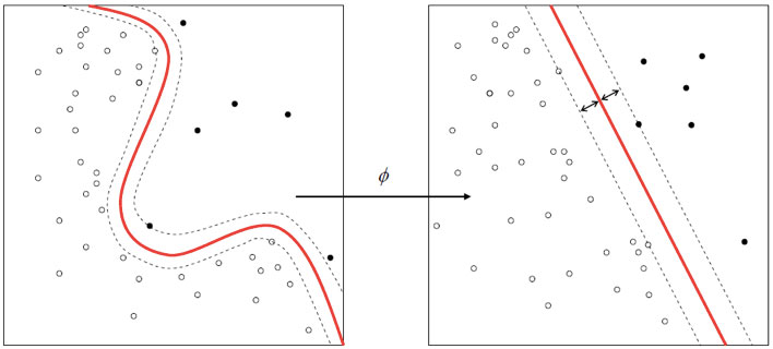
• Polynomial (homogeneous): [latex]k(\mathbf{x_i},\mathbf{x_j})=(\mathbf{x_i} \cdot \mathbf{x_j})^d[/latex]
• Polynomial (inhomogeneous): [latex]k(\mathbf{x_i},\mathbf{x_j})=(\mathbf{x_i} \cdot \mathbf{x_j} + 1)^d[/latex]
• Gaussian radial basis function: [latex]k(\mathbf{x_i},\mathbf{x_j})=\exp(-\gamma \|\mathbf{x_i}-\mathbf{x_j}\|^2)[/latex], for [latex]\gamma > 0[/latex]. Sometimes parametrized using [latex]\gamma=1/{2 \sigma^2}[/latex]
• Hyperbolic tangent: [latex]k(\mathbf{x_i},\mathbf{x_j})=\tanh(\kappa \mathbf{x_i} \cdot \mathbf{x_j}+c), for some (not every) \kappa > 0 and c < 0 [/latex]

More formally, a support vector machine constructs a hyperplane or set of hyperplanes in a high- or infinite-dimensional space, which can be used for classification, regression, or other tasks. Intuitively, a good separation is achieved by the hyperplane that has the largest distance to the nearest training-data point of any class (so-called functional margin), since in general the larger the margin the lower the generalization error of the classifier.

Whereas the original problem may be stated in a finite dimensional space, it often happens that the sets to discriminate are not linearly separable in that space. For this reason, it was proposed that the original finite-dimensional space be mapped into a much higher-dimensional space, presumably making the separation easier in that space. To keep the computational load reasonable, the mappings used by SVM schemes are designed to ensure that dot products may be computed easily in terms of the variables in the original space, by defining them in terms of a kernel function [latex]k(x,y)[/latex] selected to suit the problem. The hyperplanes in the higher-dimensional space are defined as the set of points whose dot product with a vector in that space is constant. The vectors defining the hyperplanes can be chosen to be linear combinations with parameters [latex]\alpha_i[/latex] of images of feature vectors x_i that occur in the data base. With this choice of a hyperplane, the points x in the feature space that are mapped into the hyperplane are defined by the relation: [latex]\textstyle\sum_i \alpha_i k(x_i,x) = \mathrm{constant}[/latex]. Note that if [latex]k(x,y)[/latex] becomes small as [latex]y[/latex] grows further away from [latex]x[/latex], each term in the sum measures the degree of closeness of the test point [latex]x[/latex] to the corresponding data base point [latex]x_i[/latex]. In this way, the sum of kernels above can be used to measure the relative nearness of each test point to the data points originating in one or the other of the sets to be discriminated. Note the fact that the set of points [latex]x[/latex] mapped into any hy a result, allowing much more complex discrimination between sets which are not convex at all in the original space.

Non Linear Classification

The original optimal hyperplane algorithm proposed by Vapnik in 1963 was a linear classifier. However, in 1992, Bernhard E. Boser, Isabelle M. Guyon and Vladimir N. Vapnik suggested a way to create nonlinear classifiers by applying the kernel trick (originally proposed by Aizerman et al.) to maximum-margin hyperplanes. The resulting algorithm is formally similar, except that every dot product is replaced by a nonlinear kernel function. This allows the algorithm to fit the maximum-margin hyperplane in a transformed feature space. The transformation may be nonlinear and the transformed space high dimensional; thus though the classifier is a hyperplane in the high-dimensional feature space, it may be nonlinear in the original input space.

If the kernel used is a Gaussian radial basis function, the corresponding feature space is a Hilbert space of infinite dimension. Maximum margin classifiers are well regularized, and previously it was widely believed that the infinite dimensions do not spoil the results. However, it has been shown that higher dimensions do increase the generalization error, although the amount is bounded.

Bayessian Networks.

Health Monitoring.

Our Back-Office tools introduce advanced algorithms based on Data Mining, Artificial Intelligence and Big Data techniques oriented to determine the state of the patient and prevent potential relapses and crisis.

The system can work with standard questionnaires like the PHQ-9, M.I.N.I. or Brugha, but it can be customized introducing other ones. Both the Applications and Back-Office are organized to be adapted to the required questionnaire.

The goal of the PAU is to follow the progress of the patient in the short-term, during their recovery, in order to understand behavior and give advice to patients, psychiatrists, and primary care physicians. The goal of the PU is to forecast the progress of patients some time in advance in order to detect relapses or reoccurrences by taking into account the patient assessment at current time and the knowledge obtained from data mining of previously registered major sadness data. The communication module is responsible for scheduling patients’ measurements and transmitting the results of the App to the actors involved. PAU processes all the inputs from the App by using several modules and provides the required information to patients, primary care physicians, and psychiatrists. The modules of the PAU are: the Patient Progress Module (PPM), based on a qualitative reasoning model; the Analysis Module (AM), based on expert knowledge and a rules-based system, and the Communication Module (CM).